Excelcoaching – SVerweis Formel
Den heutigen Blogeintrag möchte ich einer Excelfunktion widmen, welche auch dem nicht so geübten Exceluser leicht von der Hand geht und Zeit spart.
Mit der SVerweis Formel kann man zwei Datenbanken über einen Schlüssel miteinander vergleichen und verknüpfen.
In unserem Praxisbeispiel verwenden wir zwei Tabellen über Limonaden. Wir möchten in die Tabelle1 die Farbe der Limonade importieren, welche in der Tabelle 2 abgelegt ist.
Zieltabelle 1, hier möchten wir die Spalte C füllen mit Daten aus der Tabelle 2:
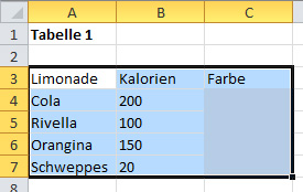
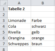
Tabelle 2, hier ist das Farbattribut, welches wir in die Spalte C in der Tabelle 1 laden möchten:
In Zelle C4 kommt nun in der Zieltabelle folgende Formel:
=SVERWEIS(A4;Tabelle2!A:B;2;FALSCH)
Dabei stehen die Werte in der Klammer (jeweils auch im Formelhelfer von Excel sichtbar) für folgendes:
A4 = Suchkriterium, nach diesem Wert wird in der Tabelle 2 gesucht
Tabelle2!A:B = Matrix, der Bereich, in welchem nach dem Wert gesucht wird und wo auch der Zielwert liegt (hier Spalte A bis B)
2 = Spaltenindex, sprich in welcher Spalte vom Anfang der Matrix gezählt das Resultat liegt (hier in der zweiten Spalte B)
falsch = Falsch gibt nur einen Wert zurück, wenn das Suchkriterium genau gefunden wird, Wahr bringt den Wert zurück, welcher dem Suchkriterium am ähnlichsten ist
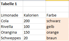
Nun kann man diese Formel mit Doppelklick auf den schwarzen Punkt, unten rechts bei der Zelle C4, ganz einfach runterkopieren in C5-C7 und erhält folgendes Resultat:
Zusammen mit der Kenntnis der F4 Funktion wie man Zellen sperrt, kann man so superschnell verknüpfte Tabellen erstellen.[:en]Today blog post I want to dedicate an Excel function that easily goes well to non experienced Excel users by the hand and saves time.
With the VLOOKUP formula, one can compare two databases on a key together and link.
In our example, we use two practice tables on sodas. We want to import in the Table 1, the color of lemonade, which is stored in table 2.
Target Table 1, here we would like to fill the column C with data from Table 2:
Today blog post I want to dedicate an Excel function that easily goes well to non experienced Excel users by the hand and saves time.
With the VLOOKUP formula, one can compare two databases on a key together and link.
In our example, we use two practice tables on sodas. We want to import in the Table 1, the color of lemonade, which is stored in table 2.
Target Table 1, here we would like to fill the column C with data from Table 2:


Table 2, here is the color attribute, which we want to load in the column C in Table 1:

In cell C4 now comes in the destination table following formula:
= VLOOKUP (A4; Table 2 A: B; 2; WRONG!)
The values are in brackets (each in the formula of Excel visible helper) for the following:
A4 = search criterion, for this value is sought in the table 2
Table 2 A: B = Matrix, the range in which to search for the value and where the target value (here column A to B)
2 = Column index, I.e. in which column counted from the beginning of the matrix, the result is (here in the second column B)
false = false is only one value if the search criterion is found exactly true brings back the value which is most similar to the search criterion
Now you can this formula by double-clicking the black dot at the bottom right of the cell C4, simply copy down in C5-C7 and get the following result:

Together with the knowledge of the F4 function to disable cell, you can create as superfast linked tables.
Table 2, here is the color attribute, which we want to load in the column C in Table 1:

In cell C4 now comes in the destination table following formula:
= VLOOKUP (A4; Table 2 A: B; 2; WRONG!)
The values are in brackets (each in the formula of Excel visible helper) for the following:
A4 = search criterion, for this value is sought in the table 2
Table 2 A: B = Matrix, the range in which to search for the value and where the target value (here column A to B)
2 = Column index, I.e. in which column counted from the beginning of the matrix, the result is (here in the second column B)
false = false is only one value if the search criterion is found exactly true brings back the value which is most similar to the search criterion
Now you can this formula by double-clicking the black dot at the bottom right of the cell C4, simply copy down in C5-C7 and get the following result:

Together with the knowledge of the F4 function to disable cell, you can create as superfast linked tables.[:]

Eine tolle Einführung in den SVerweis – hilft wirklich, Daten schnell zu verknüpfen.